#5 WayriCAD: Quick PI, Quick SI, and Thermal Checks Inside KiCad

WayriCAD, formerly KiWay, is my collection of KiCad plugins for PCB design, analysis, and project review. A growing part of that work is making electrical and thermal checks accessible while the board is still being developed: follow a power path, inspect a routed signal, or explore where heat is generated and how it leaves the board.

The three tools at the centre of that workflow are Quick PI, Quick SI, and QuickTherm. They read saved board information and combine it with explicit operating assumptions. The aim is to make those assumptions and their consequences easier to inspect, with enough context to decide what needs a closer look.

Three questions, three tools

Tool Starting question Inputs to review Results to inspect
Quick PI How much voltage is lost between the source and the load? Copper, terminals, current, material properties and returns Voltage drop, current density and copper losses
Quick SI How does a routed path compare with the signal’s edge timing? Endpoints, stackup, rise time, driver and load Delay, reflections, termination and return-path screening
QuickTherm Where does the declared dissipation go? Component powers, thermal paths, board materials and environment Component estimates and supported steady or transient board fields

Quick PI: follow the current through the copper

Quick PI starts with the saved PCB, a selected power net, and source and load terminals. The operating point includes source voltage and load current. From there, the supported DC copper models calculate voltage drop, current distribution, and resistive losses.

The simplest relationships remain useful when interpreting the maps:

\[\Delta V = I R_{\mathrm{path}}, \qquad P_{\mathrm{copper}} = I^2 R_{\mathrm{path}}.\]

Those expressions assume a fixed linear resistance. Copper geometry, thickness, conductivity, via assumptions and the selected mesh all affect the modeled path. A bright local peak is a reason to inspect the geometry and refinement, not an automatic verdict on the board.
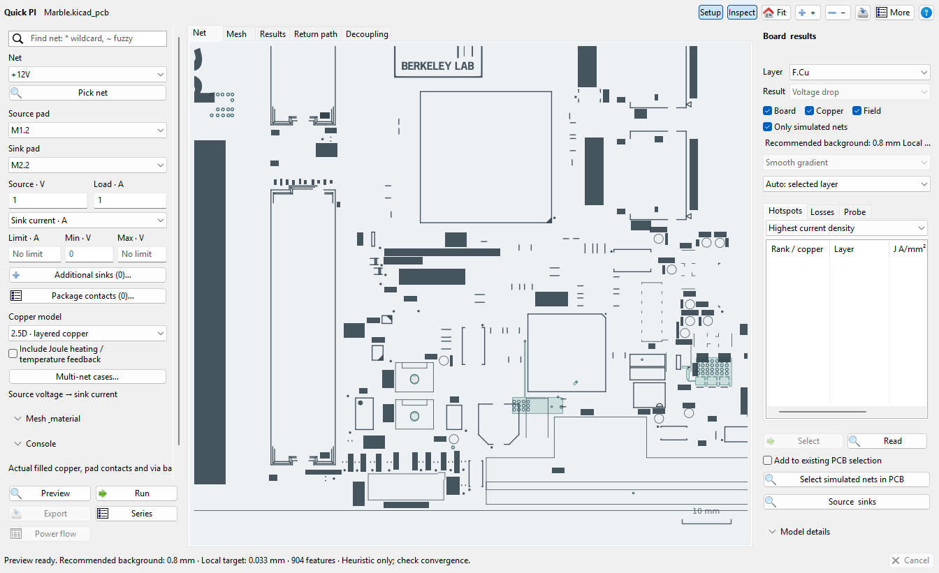
Quick PI inspecting extracted copper and source/load controls on the public Marble board
Quick PI’s native geometry preview on the public Marble board from Berkeley Lab. This capture shows extracted copper and editable inputs; no voltage field has been solved. Source and guide.

The workflow also supports multiple rails, explicit DC return copper, and grouped source/load pads. Shared-return studies solve the declared loads on common return copper together, so the return voltage drop and shared loss are accounted for explicitly. A separate geometric return-path audit answers a different question: reference coverage and transitions do not, by themselves, establish a complete electrical return circuit.

Change the load without losing the view

One recent interaction improvement is Ctrl+scroll over solved 2.5D copper to change the load current. Plain scrolling still zooms. Slow wheel movement gives finer current steps, while faster movement gives coarser changes; the plots, probes, and limits update while the view stays in place.

This reuses a fixed-temperature linear solution: voltage drop and current density scale with current, while copper loss scales with current squared. The load proportions are preserved. Changing geometry, materials, temperature, or the model itself needs the appropriate new solve; this interaction is not a substitute for an electrothermal study. The Quick PI guide describes the controls and applicability.

Quick SI: inspect the path and the assumptions together

Quick SI takes a routed signal from a source pad to a receiver pad, with the saved physical stackup and explicit driver/load assumptions. Rise time matters here: a route can be electrically significant for a fast edge even when its clock frequency seems modest.

The checks cover path delay, reflections, termination, and return-path information. The interface shows the selected route beside the assumptions and results, so you can see which path was screened and which values were supplied.
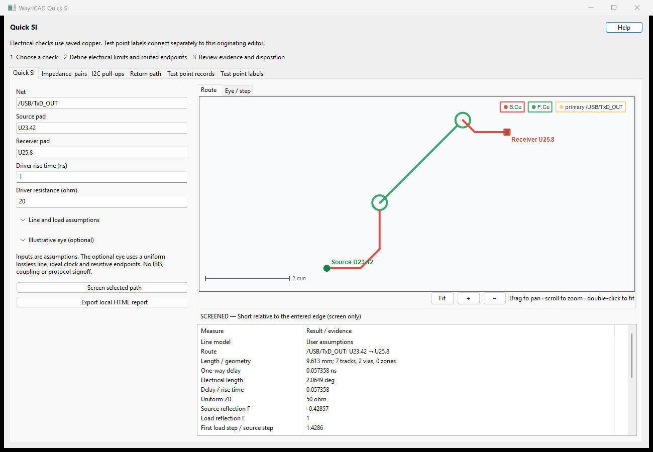
Quick SI displaying a selected routed signal, driver inputs, and a delay/reflection result table
Quick SI route inspection with entered driver and line assumptions. This is a screening workflow, not a measured channel or protocol sign-off. Guide and model details.

There is also a directed aggressor/victim workflow for supported local straight-section coupling. Its reports retain modeled coverage and omitted geometry. Local coupling results are not summed into a whole-board crosstalk prediction; branches, unsupported geometry and missing reference information still need review.

QuickTherm: start with actual dissipation

QuickTherm is installed separately from Quick PI. It reads saved footprint properties or reviewed table overrides for power, thermal resistance, and temperature limits. The important input is the component’s operating dissipation, not its maximum power rating.

At the simplest level, it provides a lumped thermal screen. Optional board models add thin-sheet or layer-resolved temperature fields, with supported steady-state and transient studies. Ambient conditions, materials, contacts and heat-rejection paths must be supplied for the selected model. Prescribed cooling conditions do not mean airflow has been solved.
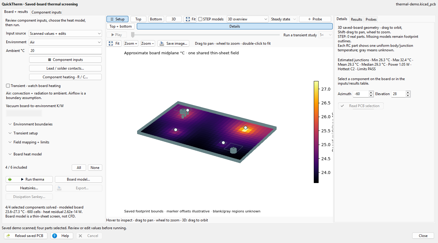
QuickTherm showing an illustrative board temperature field in its native 3D inspection view
QuickTherm’s 3D inspection of a generated thermal demonstration board under assumed loads and cooling conditions. STEP loading is off and component markers are illustrative; these are computed screening results, not measured temperatures. Capture scope and documentation.

The distinction between board temperature and package junction temperature matters. A board field does not fill in a missing package thermal path. If the selected junction model lacks the required resistance or boundary information, the result stays unknown.

Automatic mesh sizing provides a practical starting point within the model’s budget. It does not establish convergence. Local peaks still need refinement checks, and transient studies need suitable time-step checks as well. The QuickTherm user guide walks through the inputs and available models.

A workflow that keeps the context

I want these tools to fit into ordinary board development:

  1. Save the board and refill its copper zones before analyzing it.
  2. Start with one power path, signal route, or small component group.
  3. Review operating assumptions, omitted features, materials, and boundaries.
  4. Inspect the geometry alongside the plotted results and pinned probes.
  5. Compare appropriate mesh or model settings before trusting a local peak.
  6. Export the report with its inputs, coverage, warnings, and result status.

The tools support native inspection and HTML/JSON reporting, with CLI workflows for repeatable studies. Missing inputs and unsupported regions stay visible in those reports. A completed run means the selected calculation completed; its usefulness still depends on the model and the question being asked.

Beyond the quick analysis tools

WayriCAD also includes tools for fanout, via stitching, trace refinement, BOMs, assembly variants, silkscreen placement, constraints, and manufacturing review. The quick analysis tools use the same saved project alongside those design workflows.

For a broader board-and-assembly study workspace, I’m also developing SPIKE. It brings geometry, materials, study setup and results together across supported analysis workflows. It is an experimental preview; the solver documentation records the scope of each route.

Try WayriCAD

Install the tools you need through KiCad’s Plugin and Content Manager using the repository installation guide, or download packages from WayriCAD releases. The project currently documents KiCad 10 as its validated target.

The full tool catalogue and the individual PI, SI, and thermal guides are the best starting points for checking whether a particular workflow fits your board.

#4 500W Three-Phase Inverter: Architecture and Layout

This article describes the architecture and layout choices for a three-phase inverter board tested at 500 W continuous power. The main design concerns include switching loops, heat removal, gate drive, and protection.

The linked inverter board provides the project context. The sections below focus on its supporting circuits and physical layout.


System Architecture

The core topology is a three-phase, two-level voltage-source inverter (VSI). The supporting circuits handle sensing, gate drive, and filtering.

graph TD
    DC[DC Input Bus] --> Caps[DC-Link Capacitors]
    Caps --> Bridge[3-Phase VSI Bridge]
    
    MCU[Control MCU / DSP] -->|PWM Signals| Iso[Digital Isolation]
    Iso --> Gate[Isolated Gate Drivers]
    Gate -->|High/Low Side Drive| Bridge
    
    Bridge --> Filter[On-Board LC Filter]
    Filter --> Load[3-Phase Load / Motor]
    
    Bridge -.->|Current Sense| MCU
    DC -.->|Voltage Sense| MCU

The DC-link capacitor bank supplies switching current near the bridge. Excess series resistance (ESR) raises capacitor heating, while loop inductance (including capacitor ESL) contributes to voltage overshoot during switching.

The board supports multiple capacitor footprints, allowing a mix of bulk electrolytic capacitors for low-frequency energy storage and high-frequency ceramic/film capacitors placed immediately adjacent to the switching nodes.


Gate Drive and Isolation

Gate-drive timing affects switching loss, voltage overshoot, and electromagnetic interference (EMI). Faster edges can reduce transition loss but may increase ringing.

     +HV DC
       |
     | D |  (High-Side Switch)
     +---+
       |--------> Phase Output (U, V, W)
     +---+
     | D |  (Low-Side Switch)
       |
      GND

The gate-drive path uses:

  1. Digital isolators to separate control signals from the power stage.
  2. Gate drivers sized for the selected MOSFETs and switching rate.
  3. Overcurrent protection provisions, whose sensing and shutdown method depend on the final switch and driver choices.

Output Filter Design

PWM output contains switching-frequency components. Where the load or interface requires lower ripple, an output filter can attenuate those components; its values depend on the application.

This board includes on-board filter options.

  • The inductor ($L$) limits current ripple and must be checked for saturation at the expected peak current.
  • The capacitor ($C$) provides a high-frequency current path; its connection and rating depend on the chosen filter topology.

The filter is integrated on the board to keep high-frequency current paths short and make EMI easier to manage.


Physical Layout & Thermal Management

PCB layout affects voltage spikes, thermal behavior, and reliability, even when the schematic is sound.

Key Layout Principles Applied:

  1. Minimizing Commutation Loops: The loop from the DC-link capacitor, through the high-side switch, through the low-side switch, and back to the capacitor must be physically as small as possible to minimize parasitic inductance ($L_{loop}$). High $L_{loop}$ combined with high $di/dt$ causes destructive voltage spikes ($V = L \cdot di/dt$).
  2. Thermal Planes: The copper pours carrying phase currents are sized for electrical resistance and as thermal radiators.
  3. Trace Clearance: Adequate creepage and clearance distances between the high-voltage DC bus and the low-voltage control circuitry help prevent arcing.

Conclusion

The board is a test platform for motor-control and power-conversion work. Switching speed, layout, thermal design, and clearances all need to be considered together.

#3 Generating PWM with STM32

Microcontrollers handle tasks from sensor sampling to motor control. For PWM generation, the timer configuration matters as much as the application code.

For projects needing more timer channels, interfaces, or processing headroom, a 32-bit STM32 can be a useful choice. This example uses the STM32F103x8 family, which has a 72 MHz Cortex-M3 core, timers, and 12-bit ADCs; peripheral availability varies by STM32 model. See the STM32F103x8 data sheet for device limits.

View the related STM32CubeMX/HAL PWM project on GitHub

The Development Ecosystem

For an STM32F103x8 PWM project, a typical toolchain includes:

  • Software: STM32CubeMX can configure clocks and pins and generate initialization code. Keil uVision is one option for building and debugging C/C++ firmware.
  • Hardware: An ST-Link v2 can flash the device and support Serial-Wire Debugging (SWD).
  • Libraries: ST’s Hardware Abstraction Layer (HAL) can simplify setup. The timer reference manual is useful when checking update timing or debugging a configuration.

The Physical Layer of PWM

For edge-aligned PWM, the timer counts to an Auto-Reload Register (ARR) value, while a Capture/Compare Register (CCR) sets the compare point. The linked project uses STM32CubeMX and HAL; the following separate register-level illustration assumes TIM2 has a 72 MHz timer input clock and that the peripheral clock and output pin are already configured.

// Example Bare-Metal Timer Configuration
TIM2->PSC = 71;        // 72 MHz timer clock / 72 = 1 MHz tick
TIM2->ARR = 999;       // Auto-reload value (Period = 1ms -> 1kHz frequency)
TIM2->CCR1 = 500;      // Duty cycle = 50% in PWM mode 1
TIM2->CCMR1 |= TIM_CCMR1_OC1M_1 | TIM_CCMR1_OC1M_2; // PWM Mode 1
TIM2->CCER |= TIM_CCER_CC1E; // Enable Output
TIM2->CR1 |= TIM_CR1_CEN;    // Start Timer

Why It Matters in Power Electronics

Timer clock, prescaler, and register update behavior set the available PWM resolution and timing. In a power converter, also check when preload values take effect and configure dead time and protection where the switching topology requires them.

#2 Power Dissipation in Electronics: From Calculation to PCB

Power lost in a component appears mostly as heat. Estimating that loss and the path from the component to ambient helps identify where thermal validation is needed.

The Fundamentals

Power dissipation in a resistive element is:

P = I² × R  =  V² / R  =  V × I

For a 10 V to 5 V linear regulator supplying 1 A, the IC dissipates about 5 W. A buck converter delivering the same 5 W output at an assumed 90% efficiency would dissipate about 0.56 W. Actual efficiency depends on the device and operating point.

Where Power Actually Goes

In a real system, losses appear in several places:

Domain Primary Loss Mechanism
Linear regulators Voltage drop × current
MOSFETs I²×Rds(on) conduction + switching losses
Inductors I²×DCR + core losses
PCB traces I²×R_trace
Connectors Contact resistance × I²

Trace Resistance

Using bulk copper resistivity as a first estimate, a 10 mm trace that is 0.3 mm wide and 35 µm thick has:

R = ρ × L / A
R = (1.72×10⁻⁸) × 0.01 / (0.3×10⁻³ × 35×10⁻⁶)
R ≈ 16.4 mΩ

At 3 A, that is about 147 mW. Actual resistance also depends on copper thickness, temperature, and geometry.

Thermal Resistance Chain

With a heatsink, a simplified steady-state thermal path is:

T_junction = P_dissipated × (θ_jc + θ_cs + θ_sa) + T_ambient

Where:

  • θ_jc — Junction-to-case (from datasheet)
  • θ_cs — Case-to-heatsink (depends on TIM/pad)
  • θ_sa — Heatsink-to-ambient (heatsink selection)

Without a heatsink, use the package’s junction-to-ambient estimate instead of θ_sa. For example, 8 W with θ_ja = 60°C/W would imply a 480°C temperature rise in this simple model, far beyond a practical operating limit. With a heatsink and illustrative values θ_jc = 2°C/W, θ_cs = 0.5°C/W, and θ_sa = 5°C/W, the same 8 W at 40°C ambient gives an estimated junction temperature of 100°C. These values must come from the chosen device, mounting method, heatsink, and airflow. See TI’s thermal model guide for the distinction between θ_ja and a heatsink path.

My Verification Workflow

  1. Schematic phase: Annotate every power path with expected I, V, and P
  2. Layout phase: Check resistance and temperature rise on relevant power traces
  3. Thermal simulation: Build a thermal model in MATLAB or LTspice
  4. Lab validation: Thermistor + thermal camera after 30-min steady state soak

Estimate the losses, measure temperatures under representative loads, and update the model where measurements differ.

#1 Capacitive Pressure Sensing: Geometry and Readout

A capacitor’s value depends on its geometry and dielectric. If pressure deflects a diaphragm or compresses a dielectric, the resulting capacitance change can be measured. This article describes the design principle; it does not report a calibrated sensor test.

The Governing Physics

The capacitance of a parallel-plate capacitor is:

C = ε₀ × εᵣ × A / d

Where:

  • A — plate overlap area (m²)
  • d — plate separation (m)
  • εᵣ — dielectric permittivity

With a fixed plate area and dielectric, reducing a 10 µm gap to 9 µm raises the ideal parallel-plate capacitance by about 11%. Fringing fields, diaphragm shape, and material changes make the response of a real sensor less simple.

Two Structural Approaches

1. Diaphragm-Type (MEMS Style)

A thin conductive membrane is suspended over a fixed plate. Applied pressure deflects the membrane, decreasing the air gap:

ΔC / C₀ ≈ -Δd / d₀    (for small changes in gap)

MEMS devices use this principle at micrometre scale. A flexible electrode over a cavity is one possible prototype approach, but its pressure range and sensitivity depend on the mechanical design and must be calibrated.

2. Dielectric Compression

Soft dielectrics between plates may compress under load. Both gap and permittivity can change, so the capacitance-to-pressure relationship needs measurement and calibration.

Readout Circuit

One readout option converts capacitance to an oscillator frequency; the frequency equation depends on the circuit used. A capacitance-to-digital converter is another option. For example, the AD7746 data sheet specifies a ±4 pF changing-capacitance range and up to 17 pF of common-mode capacitance. Its 4 aF resolution figure describes noise under specified conditions, not overall measurement accuracy. The sensor and readout must be matched for baseline capacitance and expected change.

Noise and Stability Concerns

  • Parasitic capacitance: Keep sense connections short and consider driven guards or shielding where the readout supports them.
  • Humidity: Moisture can change dielectric properties and leakage; packaging choices depend on the intended environment.
  • Temperature drift: Characterize the sensor and readout across the operating range, then calibrate or compensate as needed.

Practical Build Notes

A prototype could use two electrodes separated by a flexible film. The next steps would be to measure baseline capacitance, apply known pressures, repeat loading cycles, and check drift and hysteresis. No pressure-to-capacitance measurement is reported here.

The geometry sets the ideal sensitivity; calibration and environmental testing determine whether a particular build is useful as a pressure sensor.